Run The Cubic Splines (Random Cubic/Linear Splines) Analysis
Mickaël Canouil, Ph.D.
Source:vignettes/articles/run-cubic-splines.Rmd
run-cubic-splines.RmdSetup
library(eggla)
#> Default 'ggplot2' theme has been changed.
#> Default 'ggplot2' colour and fill scales set to 'viridis'.
library(growthcleanr)
library(broom.mixed)
library(data.table, quietly = TRUE)

# Setup for plots
library(ggplot2, quietly = TRUE)
library(patchwork)

okabe_ito_palette <- c(
  "#E69F00FF", "#56B4E9FF", "#009E73FF", "#F0E442FF", "#0072B2FF",
  "#D55E00FF", "#CC79A7FF", "#999999FF"
)
Data
eggla includes a small dataset with 1050 rows and 6 variables.
ID(character): ID using three digits.age(numeric): age in years.sex(integer): sex with 1: male and 0: female.weight(numeric): weight in kilograms.height(integer): height in centimetres.-
bmi(numeric): Body Mass Index in kilograms per quare metre.data("bmigrowth") bmigrowth <- as.data.table(bmigrowth)bmigrowth[bmigrowth[["ID"]] == "001"] #> ID age sex weight height bmi #> <char> <num> <int> <num> <int> <num> #> 1: 001 0.00 0 3.318845 47 15.02420 #> 2: 001 0.25 0 6.585227 60 18.29230 #> 3: 001 0.50 0 7.239751 64 17.67517 #> 4: 001 0.75 0 9.474914 66 21.75141 #> 5: 001 2.00 0 13.990333 79 22.41681 #> 6: 001 4.00 0 25.909311 105 23.50051 #> 7: 001 6.00 0 30.117745 106 26.80469 #> 8: 001 12.00 0 77.958539 148 35.59101 #> 9: 001 14.00 0 92.021767 156 37.81302ggplot(data = bmigrowth) + aes(x = age, y = bmi, colour = factor(ID)) + geom_path(na.rm = TRUE, alpha = 0.25) + geom_point(size = 0.5, na.rm = TRUE, alpha = 0.25) + stat_smooth( method = "gam", formula = y ~ s(x, bs = "cr"), linetype = 1, colour = okabe_ito_palette[6], se = FALSE ) + theme(legend.position = "none") + labs(x = "AGE (years)", y = "BMI (kg/m\u00B2)") + facet_grid( cols = vars(sex), margins = TRUE, labeller = labeller( .cols = function(x) { c("0" = "FEMALE", "1" = "MALE", "2" = "FEMALE", "(all)" = "ALL")[x] } ) )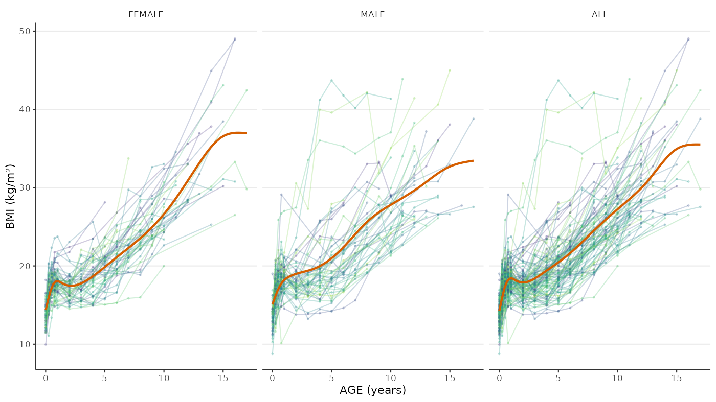
With Daymont’s QC
pheno_dt <- bmigrowth[
  j = `:=`(
    "agedays" = floor(age * 365.25), # convert to age in days and as integers ...
    "WEIGHTKG" = as.numeric(weight),
    "HEIGHTCM" = as.numeric(height)
  )
][
  j = `:=`(# recode sex with Male = 0 and Female = 1...
    "sex_daymont" = c("0" = "1", "1" = "0")[as.character(sex)]
  )
]

pheno_dt_long <- melt(
  data = pheno_dt,
  id.vars = c("ID", "age", "sex", "agedays", "sex_daymont"),
  measure.vars = c("WEIGHTKG", "HEIGHTCM"),
  variable.name = "param",
  value.name = "measurement"
)[
  j = clean := cleangrowth(# Daymont's QC from 'growthcleanr'
    subjid = ID,
    param = param,
    agedays = agedays,
    sex = sex_daymont,
    measurement = measurement,
    quietly = TRUE
  )
]
pheno_dt_clean <- dcast(
  data = pheno_dt_long[clean %in% "Include"], # Exclude all flags
  formula = ... ~ param,
  value.var = "measurement"
)[
  j = "bmi" := WEIGHTKG / (HEIGHTCM / 100)^2 # recompute bmi based using QCed variables
][
  !is.na(bmi) # exclude missing BMI related to measurements exclusion
]Modelling Female
pheno_dt_female <- pheno_dt_clean[sex_daymont == 1]
res <- egg_model(
  formula = log(bmi) ~ age, # + covariates, e.g., `log(bmi) ~ age + covariates`
  data = pheno_dt_female,
  id_var = "ID",
  random_complexity = 2, # "auto", 3, 2 or 1.
  use_car1 = TRUE # default is FALSE
)
#> Fitting model:
#>   nlme::lme(
#>     fixed = log(bmi) ~ gsp(age, knots = c(1, 8, 12), degree = rep(3, 4), smooth = rep(2, 3)),
#>     data = data,
#>     random = ~ gsp(age, knots = c(1, 8, 12), degree = rep(3, 4), smooth = rep(2, 3))[,1:3] | ID,
#>     na.action = stats::na.omit,
#>     method = "ML",
#>     correlation = nlme::corCAR1(form = ~ 1 | ID),
#>     control = nlme::lmeControl(opt = "optim", niterEM = 25, maxIter = 500, msMaxIter = 500)
#>   )
class(res)
#> [1] "lme"
sres <- tidy(res)
sres[["term"]] <- sub("gsp\\(.*\\)\\)", "gsp(...)", sres[["term"]]) # simplify output
sres
#> # A tibble: 18 × 8
#>    effect   group    term          estimate std.error    df statistic    p.value
#>    <chr>    <chr>    <chr>            <dbl>     <dbl> <dbl>     <dbl>      <dbl>
#>  1 fixed    NA       (Intercept)   2.66e+ 0   0.0323    409     82.1   2.97e-256
#>  2 fixed    NA       gsp(...)D1(…  7.37e- 1   0.113     409      6.53  1.96e- 10
#>  3 fixed    NA       gsp(...)D2(… -1.58e+ 0   0.239     409     -6.60  1.27e- 10
#>  4 fixed    NA       gsp(...)D3(…  1.62e+ 0   0.242     409      6.68  7.70e- 11
#>  5 fixed    NA       gsp(...)C(1… -1.63e+ 0   0.243     409     -6.70  7.13e- 11
#>  6 fixed    NA       gsp(...)C(8…  1.24e- 2   0.00399   409      3.12  1.97e-  3
#>  7 fixed    NA       gsp(...)C(1… -1.74e- 2   0.00990   409     -1.76  7.91e-  2
#>  8 ran_pars ID       sd_(Interce…  7.66e- 2  NA          NA     NA    NA
#>  9 ran_pars ID       cor_gsp(...… -4.82e- 1  NA          NA     NA    NA
#> 10 ran_pars ID       cor_gsp(...…  3.17e- 1  NA          NA     NA    NA
#> 11 ran_pars ID       cor_gsp(...…  3.08e- 8  NA          NA     NA    NA
#> 12 ran_pars ID       sd_gsp(...)…  2.66e- 2  NA          NA     NA    NA
#> 13 ran_pars ID       cor_gsp(...… -9.06e- 1  NA          NA     NA    NA
#> 14 ran_pars ID       cor_gsp(...… -3.86e- 8  NA          NA     NA    NA
#> 15 ran_pars ID       sd_gsp(...)…  2.76e- 3  NA          NA     NA    NA
#> 16 ran_pars ID       cor_gsp(...…  2.08e- 9  NA          NA     NA    NA
#> 17 ran_pars ID       sd_gsp(...)…  2.93e-11  NA          NA     NA    NA
#> 18 ran_pars Residual sd_Observat…  8.24e- 2  NA          NA     NA    NA
Predicted Values
ggplot() +
  aes(x = age, y = bmi) +
  geom_path(
    data = pheno_dt_female,
    mapping = aes(group = ID),
    alpha = 0.10,
    show.legend = FALSE
  ) +
  stat_smooth(
    data = pheno_dt_female,
    mapping = aes(colour = "On observed values"),
    se = FALSE,
    method = "gam",
    formula = y ~ s(x, bs = "cr")
  ) +
  stat_smooth(
    data = setnames(
      x = predict_bmi(res, start = min(pheno_dt_female[["age"]]), end = max(pheno_dt_female[["age"]])),
      old = c("egg_ageyears", "egg_bmi"),
      new = c("age", "bmi")
    ),
    mapping = aes(colour = "On predicted values"),
    se = FALSE,
    method = "gam",
    formula = y ~ s(x, bs = "cr")
  ) +
  scale_x_sqrt(
    expand = c(0, 0),
    breaks = c(0, 0.5, 1, 1.5, 2, 5, 10, 15),
    limits = c(0, NA)
  ) +
  scale_colour_manual(values = okabe_ito_palette[c(1, 2)]) +
  labs(
    x = "AGE (years)",
    y = "BMI (kg/m\u00B2)",
    colour = "GAM: y ~ s(x, bs = \"cr\")"
  ) +
  theme(
    legend.position = c(0.01, 0.99),
    legend.justification = c("left", "top")
  )
#> Warning: A numeric `legend.position` argument in `theme()` was deprecated in ggplot2
#> 3.5.0.
#> ℹ Please use the `legend.position.inside` argument of `theme()` instead.
#> This warning is displayed once every 8 hours.
#> Call `lifecycle::last_lifecycle_warnings()` to see where this warning was
#> generated.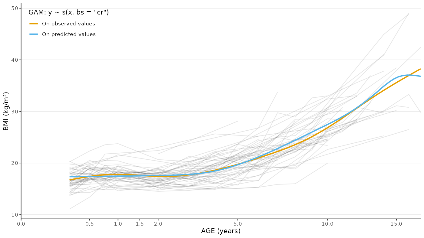
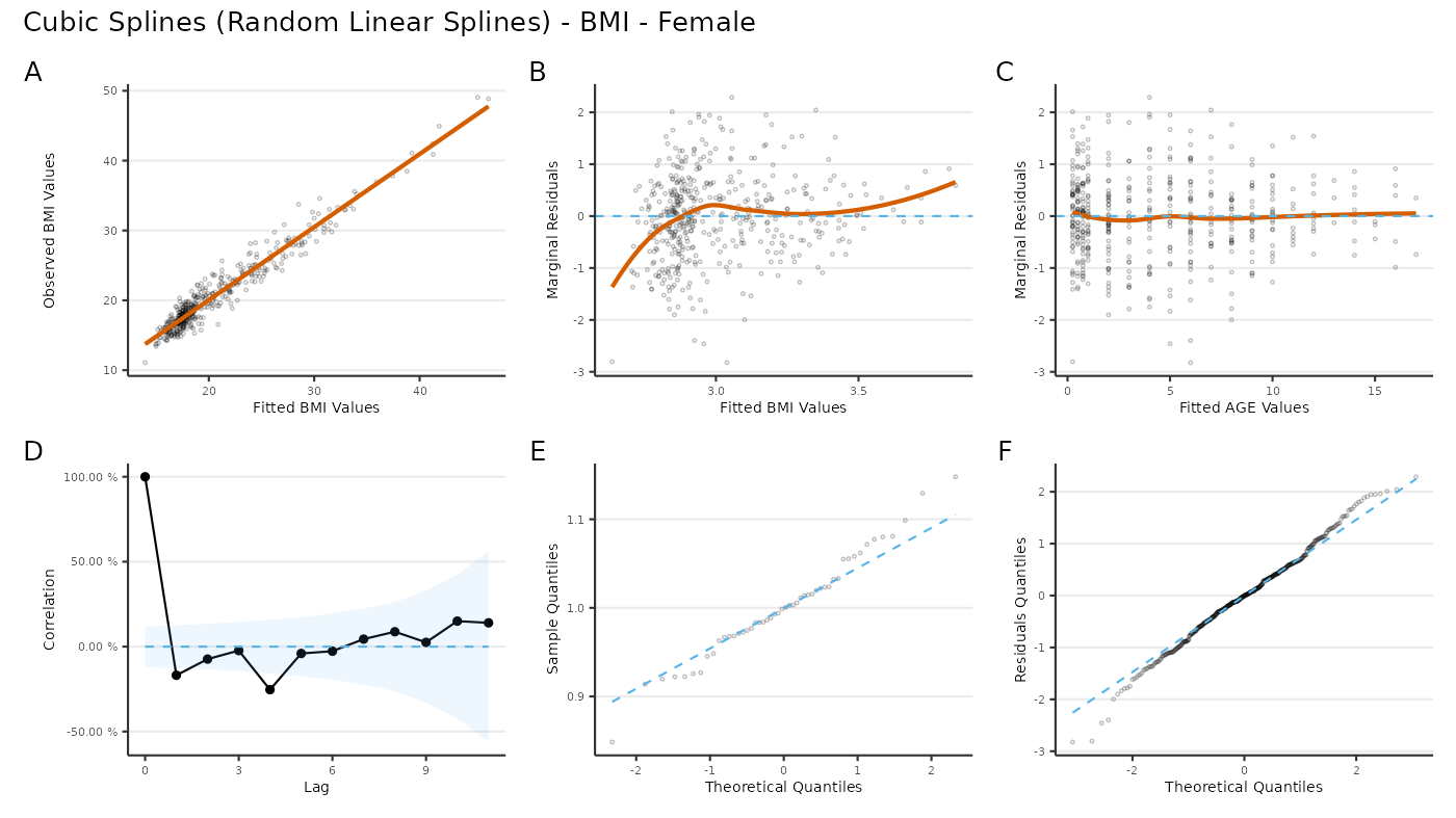
Residuals
plot_residuals(
  x = "age",
  y = "log(bmi)",
  fit = res
) +
  plot_annotation(
    title = "Cubic Splines (Random Linear Splines) - BMI - Female",
    tag_levels = "A"
  )
Predicted Average Slopes
res_pred_slopes <- egg_slopes(
  fit = res,
  period = c(0, 0.5, 1.5, 3.5, 6.5, 10, 12, 17)
)
head(res_pred_slopes)
#>    ID pred_period_0 pred_period_0.5 pred_period_1.5 pred_period_3.5
#> 1 001      2.732883        2.944564        2.957204        3.008839
#> 2 004      2.655645        2.857561        2.852242        2.874241
#> 3 005      2.617361        2.828687        2.841831        2.899329
#> 4 006      2.564983        2.770892        2.772895        2.806881
#> 5 007      2.708577        2.932235        2.967428        3.058568
#> 6 009      2.629264        2.830376        2.824291        2.848131
#>   pred_period_6.5 pred_period_10 pred_period_12 pred_period_17 slope_0--0.5
#> 1        3.212888       3.425864       3.521036       3.616467    0.4233623
#> 2        3.049543       3.252807       3.353948       3.500953    0.4038318
#> 3        3.124311       3.380123       3.508675       3.715882    0.4226518
#> 4        2.993526       3.199952       3.298031       3.421888    0.4118177
#> 5        3.307871       3.552408       3.655346       3.737519    0.4473155
#> 6        3.034627       3.263737       3.385831       3.604892    0.4022230
#>   slope_1.5--3.5 slope_6.5--10 slope_12--17
#> 1     0.02581752    0.06085040   0.01908620
#> 2     0.01099952    0.05807523   0.02940106
#> 3     0.02874899    0.07308909   0.04144143
#> 4     0.01699345    0.05897876   0.02477156
#> 5     0.04557004    0.06986760   0.01643458
#> 6     0.01192013    0.06546007   0.04381225
plot_egg_slopes(
  fit = res,
  period = c(0, 0.5, 1.5, 3.5, 6.5, 10, 12, 17)
)
#> Warning in scale_y_continuous(..., transform = transform_log10()):
#> log-10 transformation introduced infinite values.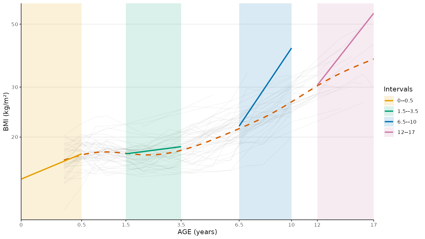
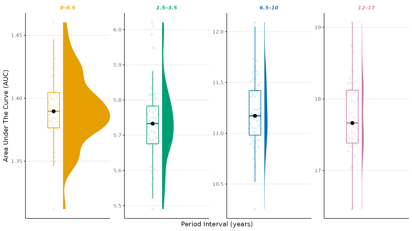
Area Under The Curve
res_auc <- egg_aucs(
  fit = res,
  period = c(0, 0.5, 1.5, 3.5, 6.5, 10, 12, 17)
)
head(res_auc)
#>      ID auc_0--0.5 auc_1.5--3.5 auc_6.5--10 auc_12--17
#> 001 001   1.431625     5.948346    11.65119   18.08524
#> 004 004   1.390543     5.707389    11.05500   17.35691
#> 005 005   1.373758     5.722382    11.41035   18.28601
#> 006 006   1.346219     5.561272    10.86764   17.02868
#> 007 007   1.422485     6.009543    12.04553   18.74309
#> 009 009   1.377140     5.652578    11.04401   17.68476
plot_egg_aucs(
  fit = res,
  period = c(0, 0.5, 1.5, 3.5, 6.5, 10, 12, 17)
)
Correlations
egg_correlations(
  fit = res,
  period = c(0, 0.5, 1.5, 3.5, 6.5, 10, 12, 17)
)
#>               term  auc_0--0.5 auc_1.5--3.5 auc_6.5--10  auc_12--17
#>             <char>       <num>        <num>       <num>       <num>
#>  1:     auc_0--0.5  1.00000000    0.7353315   0.1339844 -0.05890455
#>  2:   auc_1.5--3.5  0.73533146    1.0000000   0.7636209  0.55930196
#>  3:    auc_6.5--10  0.13398439    0.7636209   1.0000000  0.92716065
#>  4:     auc_12--17 -0.05890455    0.5593020   0.9271607  1.00000000
#>  5:   slope_0--0.5 -0.31696965    0.4092298   0.8827566  0.84524036
#>  6: slope_1.5--3.5 -0.35080310    0.3761391   0.8765640  0.87021488
#>  7:  slope_6.5--10 -0.50529328    0.1044868   0.6906018  0.88179768
#>  8:   slope_12--17 -0.24988480   -0.5206577  -0.4070861 -0.05033073
#>  9:    AP_ageyears -0.37200367    0.2662496   0.8172338  0.78849249
#> 10:    AR_ageyears  0.36773340   -0.2764872  -0.8414245 -0.83719399
#> 11:         AP_bmi  0.98613035    0.8780203   0.3266741  0.08070058
#> 12:         AR_bmi  0.84773402    0.9912778   0.6586349  0.41091288
#>     slope_0--0.5 slope_1.5--3.5 slope_6.5--10 slope_12--17 AP_ageyears
#>            <num>          <num>         <num>        <num>       <num>
#>  1:   -0.3169697     -0.3508031   -0.50529328  -0.24988480  -0.3720037
#>  2:    0.4092298      0.3761391    0.10448682  -0.52065771   0.2662496
#>  3:    0.8827566      0.8765640    0.69060183  -0.40708606   0.8172338
#>  4:    0.8452404      0.8702149    0.88179768  -0.05033073   0.7884925
#>  5:    1.0000000      0.9965866    0.80802778  -0.42159132   0.9911544
#>  6:    0.9965866      1.0000000    0.85390583  -0.34529354   0.9869343
#>  7:    0.8080278      0.8539058    1.00000000   0.19357035   0.7832160
#>  8:   -0.4215913     -0.3452935    0.19357035   1.00000000  -0.2729028
#>  9:    0.9911544      0.9869343    0.78321602  -0.27290277   1.0000000
#> 10:   -0.9969290     -0.9992709   -0.83026091   0.20818653  -0.9867121
#> 11:   -0.1848452     -0.2252452   -0.41171335  -0.36373211  -0.2175252
#> 12:    0.2043257      0.1649506   -0.08689075  -0.44388763   0.1579897
#>     AR_ageyears      AP_bmi      AR_bmi
#>           <num>       <num>       <num>
#>  1:   0.3677334  0.98613035  0.84773402
#>  2:  -0.2764872  0.87802031  0.99127780
#>  3:  -0.8414245  0.32667409  0.65863485
#>  4:  -0.8371940  0.08070058  0.41091288
#>  5:  -0.9969290 -0.18484521  0.20432572
#>  6:  -0.9992709 -0.22524516  0.16495064
#>  7:  -0.8302609 -0.41171335 -0.08689075
#>  8:   0.2081865 -0.36373211 -0.44388763
#>  9:  -0.9867121 -0.21752515  0.15798975
#> 10:   1.0000000  0.21535742 -0.17646093
#> 11:   0.2153574  1.00000000  0.91966781
#> 12:  -0.1764609  0.91966781  1.00000000
Outliers
egg_outliers(
  fit = res,
  period = c(0, 0.5, 1.5, 3.5, 6.5, 10, 12, 17),
  knots = c(1, 8, 12)
)[
  i = Outlier != 0,
  j = head(.SD),
  by = "parameter"
]
#>       parameter     ID   Row Distance_IQR Outlier_IQR Outlier
#>          <char> <char> <int>        <num>       <num>   <num>
#> 1:   auc_0--0.5    064    32     1.395147           1       1
#> 2: auc_1.5--3.5    007     5     1.307930           1       1
#> 3: auc_1.5--3.5    044    22     1.358904           1       1
#> 4:       AP_bmi    044    21     1.319709           1       1
#> 5:       AR_bmi    033    16     1.331621           1       1
#> 6:       AR_bmi    044    21     1.622874           1       1