Inline factor coercion
three or more variables
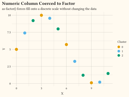
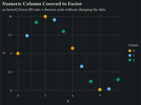
as-factor forces a numeric column to be treated as discrete for the colour aesthetic.
Late-binding aesthetics, identity scales, weights, and pipeline escape hatches.
These examples reach into the layer pipeline itself: binding aesthetics to stat outputs with after-stat, transforming resolved values with after-scale, pulling theme colours with from-theme, and splicing arbitrary closures with stat-manual. They also cover identity scales, per-row weights, factor coercion, and how reference lines interact with axis transforms. Reach for them when the standard mappings cannot express what you need; most plots never will. Every example ships its full source: click View source to copy it.
three or more variables
as-factor forces a numeric column to be treated as discrete for the colour aesthetic.
any
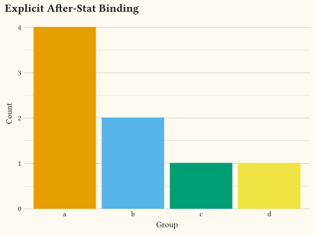
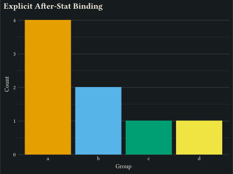
after-stat binds an aesthetic to a column produced by the layer’s stat; here y is mapped to the _count column emitted by stat-count.
any
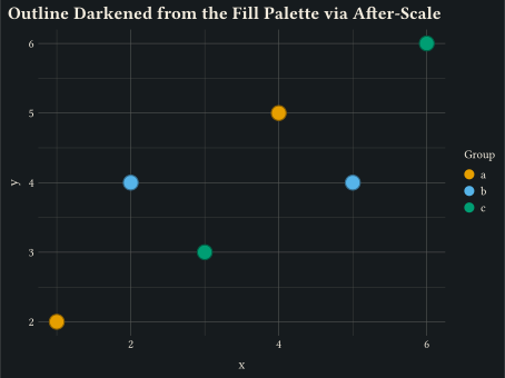
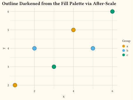
after-scale mirrors the trained fill palette into the colour channel and darkens it, so each marker outline tracks its own fill.
any
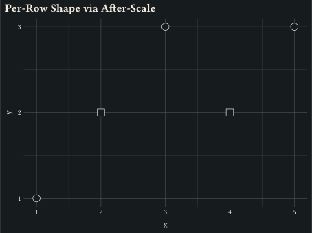
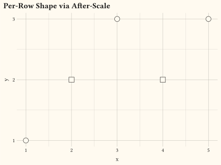
after-scale on the shape channel transforms the resolved shape kind per row, flipping between two glyphs based on a per-row predicate.
any
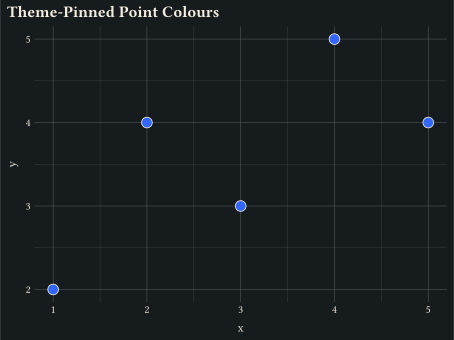
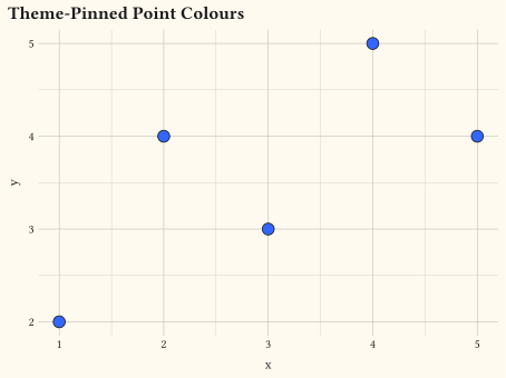
from-theme pins a layer’s stroke to the active theme’s ink and the marker fill to the accent colour, resolved once at layer prepare time.
any
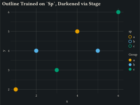
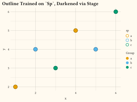
stage trains the colour aesthetic on the same column the fill scale uses, then transparentises the resolved palette swatch as the marker outline.
any
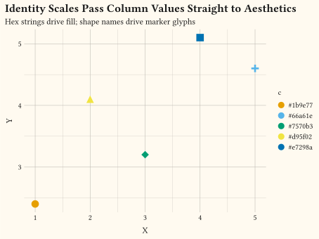
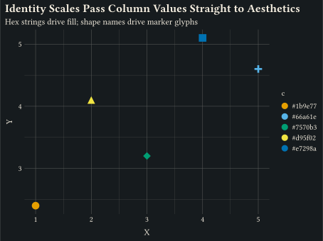
scale-identity and scale-identity pass column values directly to the visual property.
two numerics
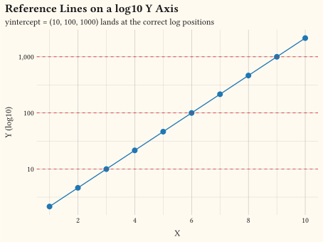
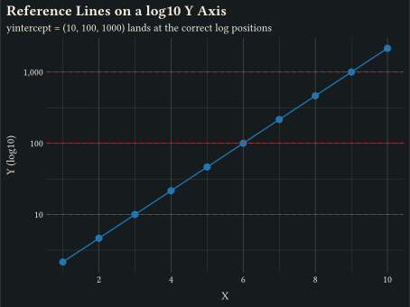
geom-hline intercepts route through the active y-axis transform so they land at the correct log positions.
two numerics
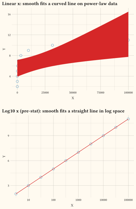
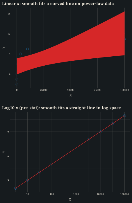
scale-log10 transforms data before stats run; geom-smooth fits the line in log space.
any
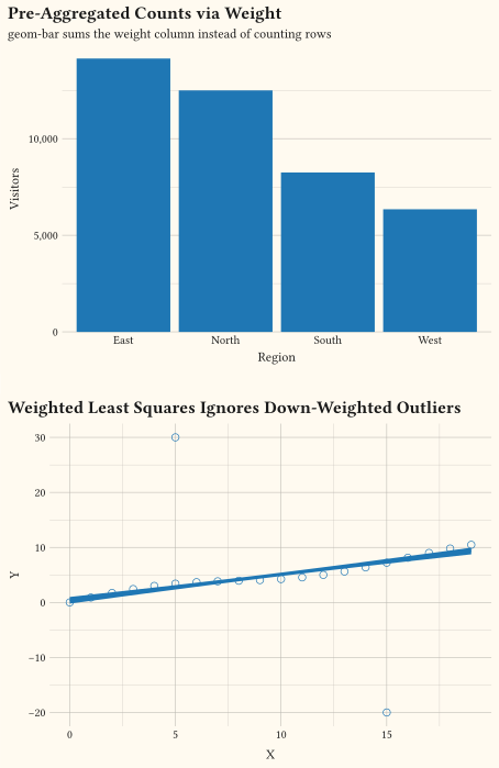
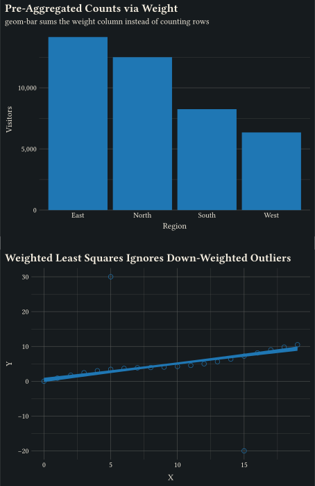
Per-row weights threaded into counts and smoothers: bars sum the weight column, weighted least squares ignores down-weighted outliers.
any
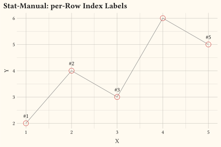
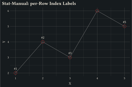
Splice a user closure into the layer pipeline via stat-manual(fun: ...); here the closure decorates each row with a per-row index used as a text label.
one numeric
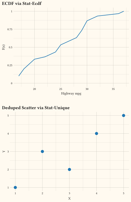
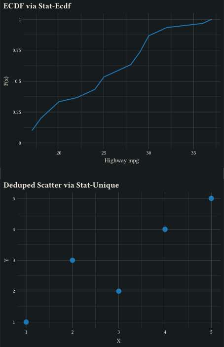
stat-ecdf draws an empirical CDF; stat-unique collapses repeated rows.
any
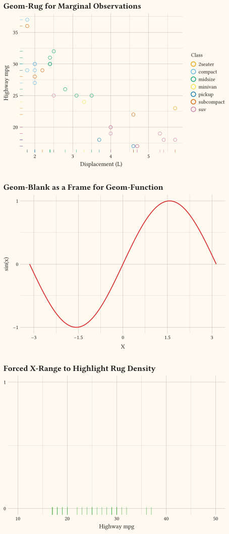
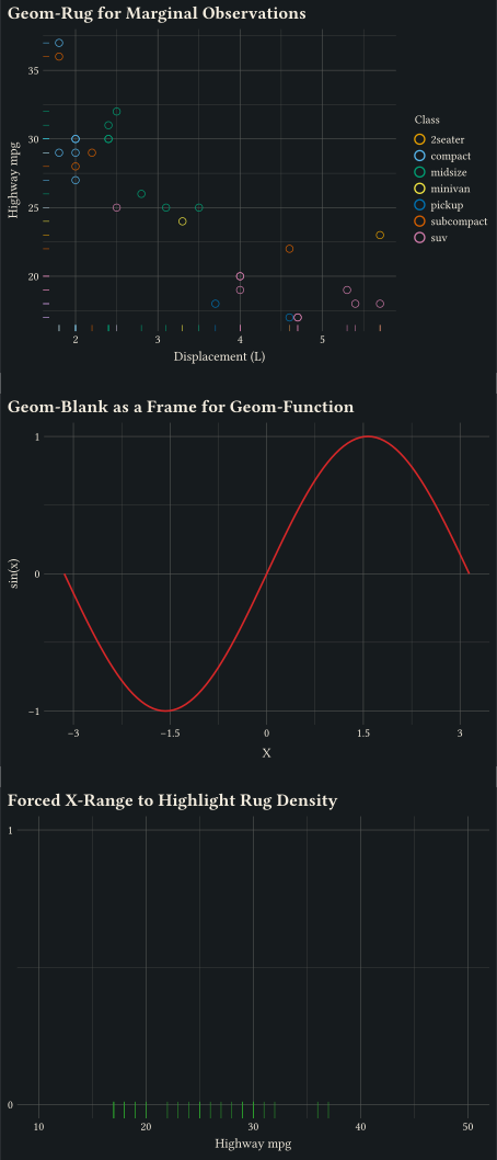
geom-rug for marginal density, geom-blank for empty frames, geom-function for analytic curves.
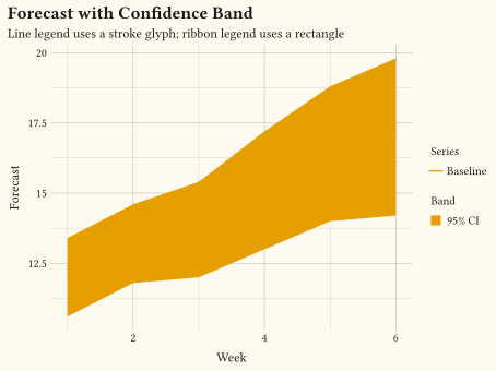
time series
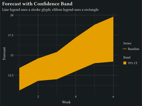
Layer geoms drive different legend glyphs: geom-line renders as a stroke, geom-ribbon as a filled rectangle.
// Inline aesthetic coercion: force a numeric column to be treated as discrete
// for the fill aesthetic without changing the underlying data.
#import "@preview/gribouille:0.7.0": *
#set page(width: auto, height: auto, margin: 0cm)
#let obs = ()
#for i in range(0, 12) {
obs.push((x: i, y: calc.sin(i / 2.0) * 5 + 5, cluster: calc.rem(i, 3)))
}
#plot(
data: obs,
mapping: aes(x: "x", y: "y", fill: as-factor("cluster")),
layers: (geom-point(size: 4pt),),
labels: labels(
title: "Numeric Column Coerced to Factor",
subtitle: "as-factor() forces fill onto a discrete scale without changing the data",
x: "X",
y: "Y",
fill: "Cluster",
),
theme: theme-minimal(),
width: 12cm,
height: 9cm,
)// `after-stat` binds an aesthetic to a column produced by the layer's
// stat. `geom-bar` runs `stat-count`, publishing `_count` per category;
// here we bind y to that column by name to make the contract explicit
// rather than relying on the geom's implicit y default. With no `labels(y:)`
// override, the y-axis title is derived from the marker: `_count` -> `Count`.
#import "@preview/gribouille:0.7.0": *
#set page(width: auto, height: auto, margin: 0cm)
#let d = (
(grp: "a"),
(grp: "b"),
(grp: "a"),
(grp: "c"),
(grp: "a"),
(grp: "b"),
(grp: "d"),
(grp: "a"),
)
#plot(
data: d,
mapping: aes(
x: "grp",
y: after-stat("_count"),
fill: "grp",
),
layers: (geom-bar(),),
guides: guides(fill: none),
labels: labels(
title: "Explicit After-Stat Binding",
x: "Group",
),
theme: theme-minimal(),
width: 12cm,
height: 9cm,
)// `after-scale` transforms an aesthetic's resolved value just before
// the geom draws. Here we mirror the trained fill palette into the
// `colour` (outline) channel and darken it, so each marker's outline
// follows its own fill swatch automatically.
#import "@preview/gribouille:0.7.0": *
#set page(width: auto, height: auto, margin: 0cm)
#let d = (
(x: 1, y: 2, sp: "a"),
(x: 2, y: 4, sp: "b"),
(x: 3, y: 3, sp: "c"),
(x: 4, y: 5, sp: "a"),
(x: 5, y: 4, sp: "b"),
(x: 6, y: 6, sp: "c"),
)
#plot(
data: d,
mapping: aes(
x: "x",
y: "y",
fill: "sp",
colour: after-scale((_, ctx) => {
let trained = ctx.trained.at("fill", default: none)
let v = ((ctx.resolve-colour)(trained, ctx.palette))(ctx.row.sp)
v.darken(40%)
}),
),
layers: (geom-point(size: 5pt, stroke: 0.8pt),),
labels: labels(
title: "Outline Darkened from the Fill Palette via After-Scale",
fill: "Group",
),
theme: theme-minimal(),
width: 12cm,
height: 9cm,
)// `after-scale` on the `shape` channel transforms the resolved shape
// kind. Here a per-row predicate flips between two shapes regardless of
// the trained shape scale.
#import "@preview/gribouille:0.7.0": *
#set page(width: auto, height: auto, margin: 0cm)
#let d = (
(x: 1, y: 1, flag: true),
(x: 2, y: 2, flag: false),
(x: 3, y: 3, flag: true),
(x: 4, y: 2, flag: false),
(x: 5, y: 3, flag: true),
)
#plot(
data: d,
mapping: aes(
x: "x",
y: "y",
shape: after-scale((_, ctx) => if ctx.row.flag { "circle" } else {
"square"
}),
),
layers: (geom-point(size: 4pt),),
labels: labels(title: "Per-Row Shape via After-Scale"),
theme: theme-minimal(),
width: 12cm,
height: 9cm,
)// Pin a layer's stroke colour to the active theme's ink and the marker
// fill to the theme's accent. `from-theme(...)` resolves once at layer
// prepare time, so the values follow whatever theme the plot picks up
// without hard-coding palette colours into the spec.
#import "@preview/gribouille:0.7.0": *
#set page(width: auto, height: auto, margin: 0cm)
#let d = (
(x: 1, y: 2),
(x: 2, y: 4),
(x: 3, y: 3),
(x: 4, y: 5),
(x: 5, y: 4),
)
#plot(
data: d,
mapping: aes(
x: "x",
y: "y",
colour: from-theme("ink"),
fill: from-theme("accent"),
),
layers: (geom-point(size: 4pt, stroke: 0.6pt),),
labels: labels(title: "Theme-Pinned Point Colours"),
theme: theme-minimal(),
width: 12cm,
height: 9cm,
)// `stage(start, after-scale)` lets the colour aesthetic train on the
// same column the fill scale uses, then transparentise the resolved
// colour palette swatch as the marker outline. The `start` column
// drives initial training; the `after-scale` closure runs per row
// after the colour scale resolves the source.
#import "@preview/gribouille:0.7.0": *
#set page(width: auto, height: auto, margin: 0cm)
#let d = (
(x: 1, y: 2, sp: "a"),
(x: 2, y: 4, sp: "b"),
(x: 3, y: 3, sp: "c"),
(x: 4, y: 5, sp: "a"),
(x: 5, y: 4, sp: "b"),
(x: 6, y: 6, sp: "c"),
)
#plot(
data: d,
mapping: aes(
x: "x",
y: "y",
fill: "sp",
colour: stage(
start: "sp",
after-scale: (c, _) => c.darken(40%),
),
),
layers: (geom-point(size: 5pt, stroke: 0.8pt),),
labels: labels(
title: "Outline Trained on `Sp`, Darkened via Stage",
fill: "Group",
),
theme: theme-minimal(),
width: 12cm,
height: 9cm,
)// Identity scales: the column value IS the visual property.
#import "@preview/gribouille:0.7.0": *
#set page(width: auto, height: auto, margin: 0cm)
#let signals = (
(x: 1, y: 2.4, c: "#1b9e77", s: "circle"),
(x: 2, y: 4.1, c: "#d95f02", s: "triangle"),
(x: 3, y: 3.2, c: "#7570b3", s: "diamond"),
(x: 4, y: 5.1, c: "#e7298a", s: "square"),
(x: 5, y: 4.6, c: "#66a61e", s: "cross"),
)
#plot(
data: signals,
mapping: aes(x: "x", y: "y", fill: "c", shape: "s"),
layers: (geom-point(size: 4pt),),
scales: scales(colour: scale-identity(), shape: scale-identity()),
labels: labels(
title: "Identity Scales Pass Column Values Straight to Aesthetics",
subtitle: "Hex strings drive fill; shape names drive marker glyphs",
x: "X",
y: "Y",
),
theme: theme-minimal(),
width: 12cm,
height: 9cm,
)// Reference lines on a log10 y axis: yintercept values land at the correct
// log positions because hline routes through the axis transform.
#import "@preview/gribouille:0.7.0": *
#set page(width: auto, height: auto, margin: 0cm)
#let accent = rgb("#1f77b4")
#let df = range(1, 11).map(i => (x: i, y: calc.pow(10, i / 3)))
#plot(
data: df,
mapping: aes(x: "x", y: "y"),
layers: (
geom-line(stroke: 1pt, colour: accent, alpha: 0.5),
geom-point(size: 3pt, fill: accent),
geom-hline(
yintercept: (10, 100, 1000),
colour: rgb("#d62728"),
linetype: "dashed",
),
),
scales: scales(y: scale-log10(labels: format-comma())),
labels: labels(
title: "Reference Lines on a log10 Y Axis",
subtitle: "yintercept = (10, 100, 1000) lands at the correct log positions",
x: "X",
y: "Y (log10)",
),
theme: theme-minimal(),
width: 12cm,
height: 9cm,
)// scale_x_log10 pre-transforms data: stats fit a line in log space, so a
// power-law dataset comes out straight.
#import "@preview/gribouille:0.7.0": *
#set page(width: auto, height: auto, margin: 0cm)
#let accent = rgb("#1f77b4")
#let red = rgb("#d62728")
#let d = range(1, 11).map(i => (x: calc.pow(10, i / 2), y: 2 * (i / 2) + 1))
#let panel(title, scales) = plot(
data: d,
mapping: aes(x: "x", y: "y"),
layers: (
geom-point(size: 3pt, colour: accent),
geom-smooth(method: "lm", colour: red, fill: red, alpha: 0.15),
),
scales: scales,
labels: labels(title: title, x: "X", y: "Y"),
theme: theme-minimal(),
width: 12cm,
height: 9cm,
)
#grid(
columns: 1,
row-gutter: 0.5cm,
panel("Linear x: smooth fits a curved line on power-law data", (:)),
panel(
"Log10 x (pre-stat): smooth fits a straight line in log space",
scales(x: scale-log10()),
),
)// weight aesthetic: per-row weights threaded into counts, bins, and smoothers.
#import "@preview/gribouille:0.7.0": *
#set page(width: auto, height: auto, margin: 0cm)
#let accent = rgb("#1f77b4")
#let totals = (
(region: "North", visitors: 12450),
(region: "South", visitors: 8200),
(region: "East", visitors: 14100),
(region: "West", visitors: 6300),
)
#let bars = plot(
data: totals,
mapping: aes(x: "region", weight: "visitors"),
layers: (geom-bar(fill: accent),),
scales: scales(y: scale-continuous(labels: format-comma())),
labels: labels(
title: "Pre-Aggregated Counts via Weight",
subtitle: "geom-bar sums the weight column instead of counting rows",
x: "Region",
y: "Visitors",
),
theme: theme-minimal(),
width: 12cm,
height: 9cm,
)
#let pts = ()
#for i in range(0, 20) {
pts.push((x: i, y: i * 0.5 + calc.sin(i * 0.4), w: 1))
}
// Two outliers with negligible weight: WLS pulls the fit back to the trend.
#pts.push((x: 5, y: 30, w: 0.001))
#pts.push((x: 15, y: -20, w: 0.001))
#let scatter = plot(
data: pts,
mapping: aes(x: "x", y: "y", weight: "w"),
layers: (
geom-point(size: 2.5pt, alpha: 0.8, colour: accent),
geom-smooth(method: "lm", colour: accent, fill: accent, alpha: 0.2),
),
labels: labels(
title: "Weighted Least Squares Ignores Down-Weighted Outliers",
x: "X",
y: "Y",
),
theme: theme-minimal(),
width: 12cm,
height: 9cm,
)
#grid(
columns: 1,
row-gutter: 0.5cm,
bars,
scatter,
)// stat-manual lets you splice an ad-hoc closure into the layer pipeline.
// Here it adds a per-row index column, drawn as text labels.
#import "@preview/gribouille:0.7.0": *
#set page(width: auto, height: auto, margin: 0cm)
#let d = (
(x: 1, y: 2),
(x: 2, y: 4),
(x: 3, y: 3),
(x: 4, y: 6),
(x: 5, y: 5),
)
#let with-index = data => (
data
.enumerate()
.map(((i, r)) => (
r
+ (
label: "#" + str(i + 1),
)
))
)
#plot(
data: d,
mapping: aes(x: "x", y: "y"),
layers: (
geom-line(stroke: 0.6pt, colour: rgb("#888")),
geom-point(size: 4pt, colour: rgb("#cc3333")),
geom-text(
mapping: aes(label: "label", nudge-y: 0.4cm),
stat: stat-manual(fun: with-index),
size: 9pt,
),
),
labels: labels(title: "Stat-Manual: per-Row Index Labels", x: "X", y: "Y"),
theme: theme-minimal(),
width: 12cm,
height: 8cm,
)// stat-ecdf and stat-unique: ECDF curve plus a deduplicated scatter.
#import "@preview/gribouille:0.7.0": *
#set page(width: auto, height: auto, margin: 0cm)
#let accent = rgb("#1f77b4")
#let ecdf = plot(
data: mpg,
mapping: aes(x: "hwy"),
layers: (geom-line(stat: "ecdf", colour: accent, stroke: 1.4pt),),
scales: scales(x: scale-continuous(name: "Highway mpg"), y: scale-continuous(name: "F(x)", limits: (0, 1))),
labels: labels(
title: "ECDF via Stat-Ecdf",
x: "Highway mpg",
y: "F(x)",
),
theme: theme-minimal(),
width: 12cm,
height: 9cm,
)
#let scatter = (
(x: 1, y: 1),
(x: 1, y: 1),
(x: 1, y: 1),
(x: 2, y: 3),
(x: 2, y: 3),
(x: 3, y: 2),
(x: 4, y: 4),
(x: 4, y: 4),
(x: 5, y: 5),
)
#let dedup = plot(
data: scatter,
mapping: aes(x: "x", y: "y"),
layers: (geom-point(stat: "unique", size: 4pt, fill: accent),),
labels: labels(title: "Deduped Scatter via Stat-Unique", x: "X", y: "Y"),
theme: theme-minimal(),
width: 12cm,
height: 9cm,
)
#grid(
columns: 1,
row-gutter: 0.6cm,
ecdf,
dedup,
)// Long-tail geoms: blank, rug, function across three panels.
#import "@preview/gribouille:0.7.0": *
#set page(width: auto, height: auto, margin: 0cm)
#let p1 = plot(
data: mpg,
mapping: aes(x: "displ", y: "hwy", colour: "class"),
layers: (
geom-point(size: 2.5pt, alpha: 0.85),
geom-rug(sides: "bl"),
),
labels: labels(
title: "Geom-Rug for Marginal Observations",
x: "Displacement (L)",
y: "Highway mpg",
colour: "Class",
),
theme: theme-minimal(),
width: 12cm,
height: 9cm,
)
#let frame = ((x: -calc.pi, y: -1), (x: calc.pi, y: 1))
#let p2 = plot(
data: frame,
mapping: aes(x: "x", y: "y"),
layers: (
geom-blank(),
geom-function(
fun: x => calc.sin(x),
x-limits: (-calc.pi, calc.pi),
colour: rgb("#d62728"),
stroke: 1.2pt,
),
),
scales: scales(x: scale-continuous(breaks: (-3, -1.5, 0, 1.5, 3))),
labels: labels(
title: "Geom-Blank as a Frame for Geom-Function",
x: "X",
y: "sin(x)",
),
theme: theme-minimal(),
width: 12cm,
height: 9cm,
)
#let p3 = plot(
data: mpg,
mapping: aes(x: "hwy"),
layers: (
geom-blank(
data: ((x: 10, y: 0), (x: 50, y: 1)),
mapping: aes(x: "x", y: "y"),
inherit-aes: false,
),
geom-rug(sides: "b", colour: rgb("#2ca02c"), length: 0.4cm),
),
scales: scales(x: scale-continuous(name: "Highway mpg")),
labels: labels(title: "Forced X-Range to Highlight Rug Density", y: none),
theme: theme-minimal(),
width: 12cm,
height: 9cm,
)
#grid(
columns: 1,
row-gutter: 0.5cm,
p1,
p2,
p3,
)// Per-geom legend glyphs: line layers contribute strokes, ribbon layers
// contribute filled rectangles, so the `colour` and `fill` aesthetics each
// resolve to the right glyph automatically.
#import "@preview/gribouille:0.7.0": *
#set page(width: auto, height: auto, margin: 0cm)
#let forecast = (
(week: 1, fit: 12.0, lo: 10.6, hi: 13.4, band: "95% CI", series: "Baseline"),
(week: 2, fit: 13.2, lo: 11.8, hi: 14.6, band: "95% CI", series: "Baseline"),
(week: 3, fit: 13.7, lo: 12.0, hi: 15.4, band: "95% CI", series: "Baseline"),
(week: 4, fit: 15.1, lo: 13.0, hi: 17.2, band: "95% CI", series: "Baseline"),
(week: 5, fit: 16.4, lo: 14.0, hi: 18.8, band: "95% CI", series: "Baseline"),
(week: 6, fit: 17.0, lo: 14.2, hi: 19.8, band: "95% CI", series: "Baseline"),
)
#plot(
data: forecast,
mapping: aes(x: "week", y: "fit", colour: "series", fill: "band"),
layers: (
geom-ribbon(
mapping: aes(ymin: "lo", ymax: "hi"),
alpha: 0.3,
inherit-aes: true,
),
geom-line(stroke: 1.2pt),
),
scales: scales(x: scale-continuous(name: "Week"), y: scale-continuous(name: "Forecast", labels: format-comma())),
labels: labels(
title: "Forecast with Confidence Band",
subtitle: "Line legend uses a stroke glyph; ribbon legend uses a rectangle",
colour: "Series",
fill: "Band",
),
theme: theme-minimal(),
width: 12cm,
height: 9cm,
)