stat-density-2d
2D density statistic: iso-lines of a Gaussian kernel density estimate.
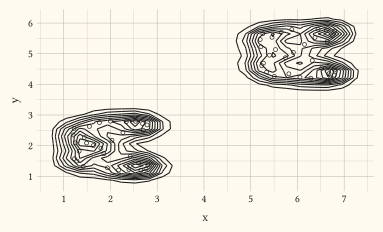
Smooths the (x, y) sample into a density surface on an n × n grid, then traces the surface’s contour lines. Emits the same row shape as stat-contour (x, y, group, _level), so it pairs with geom-density-2d or geom-path.
Either breaks, binwidth, or bins controls level placement; precedence runs breaks > binwidth > bins (default bins: 10).
from R’s bw.nrd / 4 (the seed MASS kde2d uses); pass a number for both axes or an (x, y) tuple.
Usage
stat-density-2d(
  bw: auto,
  adjust: 1,
  n: 25,
  bins: 10,
  binwidth: none,
  breaks: auto,
)
Parameters
| Parameter | Default | Description |
|---|---|---|
bw |
auto |
Kernel standard deviation per axis. auto derives it per axis |
adjust |
1 |
Bandwidth multiplier: adjust: 0.5 halves the smoothing. |
n |
25 |
Grid resolution per axis: a number or an (x, y) tuple. |
bins |
10 |
Target contour-level count when breaks and binwidth are unset. |
binwidth |
none |
Fixed step between levels. Overrides bins. |
breaks |
auto |
Explicit array of contour levels. Overrides bins and binwidth. |
Returns
Statistic object with name: "density-2d".
Outputs
x.y.group._level.
Examples
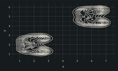
Density contours of two point clouds via geom-path.
#let d = range(0, 60).map(i => {
  let lobe = calc.rem(i, 2)
  (
    x: 2 + lobe * 4 + calc.sin(i * 1.7) * 0.8,
    y: 2 + lobe * 3 + calc.cos(i * 2.3) * 0.8,
  )
})
#plot(
  data: d,
  mapping: aes(x: "x", y: "y"),
  layers: (
    geom-point(size: 1.5pt, alpha: 0.5),
    geom-path(stat: stat-density-2d(bins: 8)),
  ),
  width: 10cm,
  height: 6cm,
)