stat-ydensity
Y-density statistic: Gaussian kernel density estimate of y per x bucket.
For every distinct x value, emits n evenly spaced rows along y where violinwidth is the display width in [0, 1], plus the after-stat columns _density (estimated density), _count (density scaled by the bucket’s observation count), _scaled (density scaled to a per-bucket maximum of 1), and _n (the bucket’s observation count).
Widths are normalised across the buckets of one aesthetic group; with a colour/fill grouping each group normalises independently.
(R’s bw.nrd0); pass a positive number to fix it.
adjust: 0.5 halves the smoothing.
per bucket.
true (default) trims the tails; false extends the grid by three bandwidths on each side.
divides every density by the largest density so equal areas read as equal mass, "count" additionally weights each bucket by its observation count, and "width" stretches every bucket to the full width.
Usage
stat-ydensity(
  bw: auto,
  adjust: 1,
  n: 512,
  trim: true,
  scale: "area",
)
Parameters
| Parameter | Default | Description |
|---|---|---|
bw |
auto |
Kernel bandwidth. auto applies Silverman’s rule of thumb |
adjust |
1 |
Bandwidth multiplier: the kernels use adjust * bw, so |
n |
512 |
Number of evenly spaced grid points the density is evaluated at |
trim |
true |
Whether to restrict each curve to its bucket’s y range. |
scale |
"area" |
Width normalisation across buckets. "area" (default) |
Returns
Statistic object with name: "ydensity", consumed by geom-violin.
Outputs
x.y.violinwidth._density._count._scaled._n.
Examples
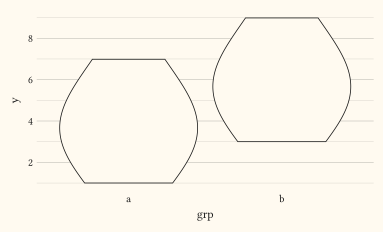
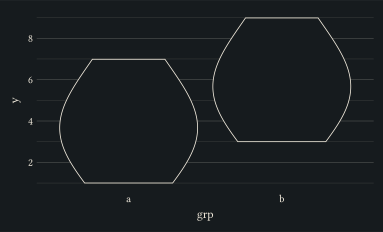
Wider smoothing via adjust on the backing statistic.
#let ys = (1, 2, 2, 3, 4, 4, 4, 5, 6, 7)
#let d = ()
#for grp in ("a", "b") {
  for y in ys {
    d.push((grp: grp, y: y + (if grp == "b" { 2 } else { 0 })))
  }
}
#plot(
  data: d,
  mapping: aes(x: "grp", y: "y"),
  layers: (geom-violin(stat: stat-ydensity(adjust: 2)),),
  width: 10cm,
  height: 6cm,
)