stat-density
Density statistic: Gaussian kernel density estimate of the x sample.
Emits n evenly spaced (x, y) rows per group where y is the estimated density, plus the after-stat columns _density (same as y), _count (density scaled by the number of observations), _scaled (density scaled to a maximum of 1), and _n (the number of observations).
(R’s bw.nrd0); pass a positive number to fix it.
adjust: 0.5 halves the smoothing.
(default) extends it by three bandwidths on each side so the curve decays to the baseline.
Usage
stat-density(
  bw: auto,
  adjust: 1,
  n: 512,
  trim: false,
)
Parameters
| Parameter | Default | Description |
|---|---|---|
bw |
auto |
Kernel bandwidth. auto applies Silverman’s rule of thumb |
adjust |
1 |
Bandwidth multiplier: the kernels use adjust * bw, so |
n |
512 |
Number of evenly spaced grid points the density is evaluated at. |
trim |
false |
Whether to restrict the grid to the data range. false |
Returns
Statistic object with name: "density", consumed by geom layers.
Outputs
x.y._density._count._scaled._n.
Examples
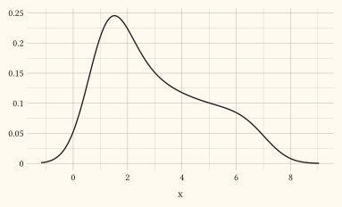
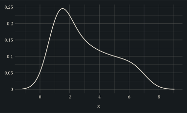
Density curve of a skewed sample via geom-line(stat: "density").
#let d = range(0, 60).map(i => (
  x: calc.pow(calc.rem(i * 7, 30) / 10, 2) * 0.7 + 1,
))
#plot(
  data: d,
  mapping: aes(x: "x"),
  layers: (geom-line(stat: "density", stroke: 1pt),),
  width: 10cm,
  height: 6cm,
)
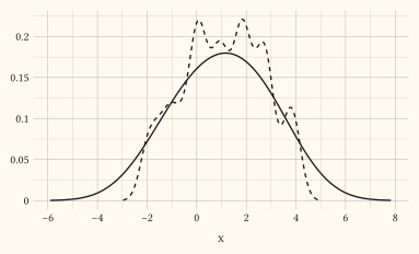
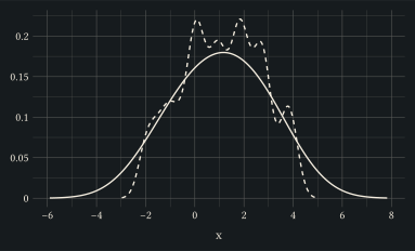
Constructor form: customise the smoothing with adjust on any geom; here a coarser and a finer estimate of the same sample overlay.
#let d = range(0, 60).map(i => (
  x: calc.sin(i * 0.9) * 2 + calc.rem(i, 3),
))
#plot(
  data: d,
  mapping: aes(x: "x"),
  layers: (
    geom-line(stat: stat-density(adjust: 2), stroke: 1pt),
    geom-line(stat: stat-density(adjust: 0.5), stroke: 1pt, linetype: "dashed"),
  ),
  width: 10cm,
  height: 6cm,
)